Parameter guide

There are a bunch of parameters that impact the visualization quality of t-SimCNE. Some parameters are straightforward to interpret but some can have subtle influences on the quality. Here we aim to point out some knobs that you can turn along with what you can expect to change.

Here we only present a selection of all of the parameters. The full list with the documentation is in the t-SimCNE API reference.

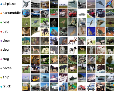
All of the examples here are done on the CIFAR-10 dataset, which is a simple image dataset. For your convenience, here is a small legend with sample pictures.

Number of epochs

One of the most intuitive parameters is the number of epochs, controlled by the parameter total_epochs. It is a list with three numbers, corresponsing to the number of epochs per dimension. The fewer epochs we have, the faster the model will be trained, but at the expense of the embedding quality.

In this case we have three separate stages in which we train, hence we can change the number of epochs in three different places.

The first stage is the high-dimensional pretraining. This will learn a good representation in a 128D space. The second stage will be a short transitional stage down to 2D where we have most of the network frozen and only train the last layer (which is initialized only at this stage). Afterwards we do the fine-tuning with the whole network.

By default we have the following number of epochs for the three stages:

• 1000 epochs high-dimensional pretraining

• 50 epochs 2D linear layer training

• 450 epochs finetuning the whole network in 2D

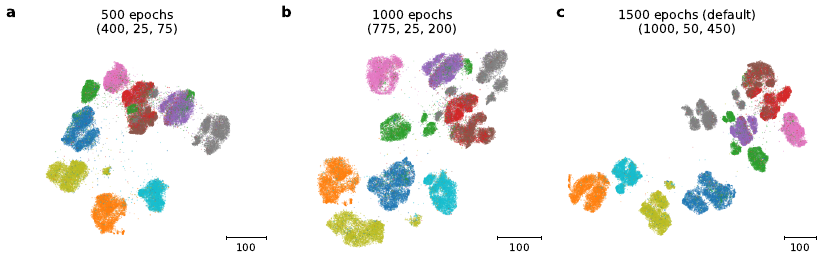
By decreasing the number of epochs, we can speed up the computation but risk getting a worse embedding quality. For reference, here are some different settings for the number of epochs.

a = TSimCNE(total_epochs=[400, 25, 75])
b = TSimCNE(total_epochs=[775, 25, 200])
c = TSimCNE()

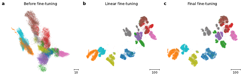
To see how the intermediate visualization looks, we can also extract the embedding at three points in the optimization process, which gives a hint as to what is being changed in the visualization.

In the image below we can see that the macro scale is mostly set already even before we start the second optimization stage (the last linear layer was randomly initialized, but not yet optimized). The second stage manages to bring out most of the structure already and shows clear similarity to the final visualization. The last stage is more concerned with detail work and the micro-scale structure. For example the grey cluster (corresponsing to horse pictures) in the upper part is better separated in panel c compared to panel b.

Batch size

The batch_size is a parameter that should usually be set as large as the GPU memory allows. This is due to contrastive learning requiring a large batch in order to have enough representative samples for calculating the alignment and uniformity. The default is simply set to 512; in the paper we used 1024. (For CIFAR-sized datasets this could probably also be set lower than 512.)

There is quite a bit of literature on this and the effect of the batch size in the contrastive learning setting it still ongoing research. The first paper on contrastive learning had already pointed out that performance increases with largeger batch size for SimCLR (Chen et al., ICML 2020).

Output dimension

The output dimension is set to 2 so that we can straightforwardly visualize the result. But we could, for example, also visualize the result in three dimensions or use even more dimensions to facilitate some downstream analysis. For this we provide the parameter out_dim.

t = TSimCNE(out_dim=3)
Y = t.fit_transform(X)

A t-SimCNE visualization in 3D of the CIFAR-10 dataset.

Network model

The model can of course also be changed. In the paper we limit ourselves to the same ResNet18 architecture as described in the SimCLR paper (which has a smaller kernel size in the first conv block). But the backbone of the network can be changed to anything else that makes sense for your application. Some ideas would be to use a more efficient network such as EfficientNet or MobileNet v3. You could also use an already pretrained network, which can speed up the training.

t = TSimCNE(backbone="resnet50")
Y = t.fit_transform(X)

Note

The hyperparameters need to be tuned separately for other backbones, the default is supposed to work well with resnet18.

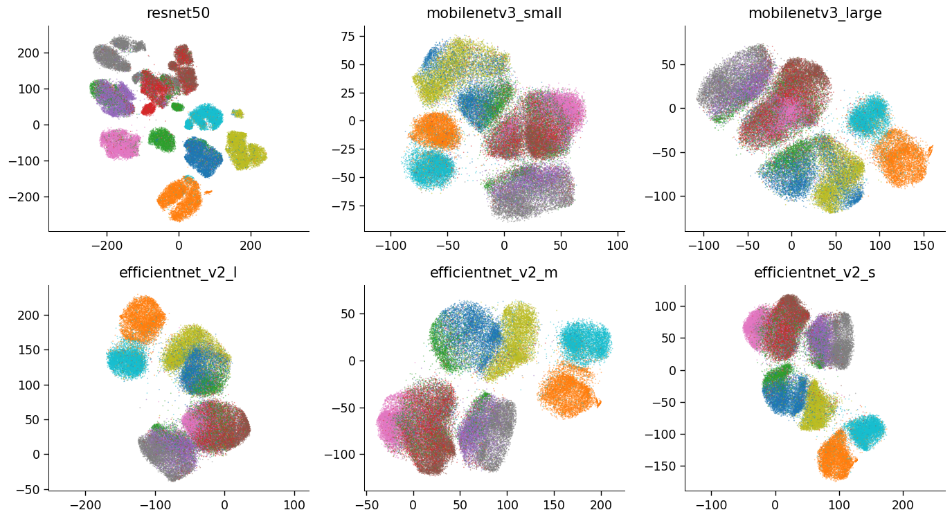
Different backbones trained on CIFAR-10.

The projection head can also be changed, although the implications of this are quite hard to predict. Hence, we recommend to leave this as is (adjusting for the changed output dimension though, should this change in the backbone).

If the parameter model is passed to the network, then both the backbone and projection_head parameters will be ignored.

Currently the backbones that can be passed in as keywords are the following. Note that the stride is changed in resnet18 and well as all of the mobilenetv3 and efficientnet models, akin to the SimCLR paper.

• "resnet18"

• "resnet34"

• "resnet50"

• "resnet101"

• "mobilenetv3_small"

• "mobilenetv3_large"

• "efficientnet_v2_s"

• "efficientnet_v2_m"

• "efficientnet_v2_l"

FFCV data loading

There is also the option to use FFCV for loading the data, resulting in faster loading time. This is an optional feature and the library is not installed by default (since it proved surprisingly difficult to install it directly without issues).

After installation, to use FFCV, simply pass in the size of the images and the path to the .beton file (which needs to have been prepared in advance, see “Writing a dataset to FFCV format”).

t = TSimCNE(image_size=(32, 32))
Y = t.fit_transform("cifar10.beton")

The data should load faster compared to using a regular torch dataset. To use the functionality, you need to have FFCV-SSL (Bordes et al., 2023) installed, since plain FFCV does not support all of the required functionality for contrastive learning.

Speedup

The speedup on CIFAR datasets is around 25% (with the default pytorch dataset one epoch takes ~25 seconds; with FFCV it takes ~20 seconds). Be aware that the improvement will probably be better for larger images and it always depends on your GPU and computer architecture. So take the 25% speedup more as a rough estimate.